A scientific calculator fits in your pocket, runs on a tiny battery, and can instantly compute the sine of an angle, the natural logarithm of a number, or the root of a complex expression. This article goes deep from the physical keypress all the way to the algorithm that computes trigonometric functions using nothing but addition and bit-shifting. If you use our Videnskabelig Lommeregner, this is exactly how it works under the hood.
1. A Brief History: From Gears to Silicon
The story of the calculator begins in 1623, when Wilhelm Schickard of Tübingen built the first known mechanical calculator. Nine years later, Blaise Pascal invented the Pascaline, a brass machine that could add and subtract through an ingenious carry mechanism. Gottfried Wilhelm Leibniz refined these ideas in the 1670s with his Stepped Reckoner, introducing the drum gear that allowed multiplication and division.
The leap to electronics came in 1961 with the ANITA Mark VII the world’s first all-electronic desktop calculator. Texas Instruments introduced mass-produced integrated-circuit calculators in 1965, making them affordable and reliable.
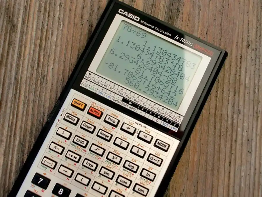
The defining moment for scientific calculators arrived in 1972, when Hewlett-Packard released the HP-35 the world’s first handheld scientific calculator. Named for its 35 keys, it weighed 255 grams, ran on a rechargeable battery, and could perform trigonometric, logarithmic, and exponential functions. Priced at $395, market researchers warned HP it would never sell. In its first year, HP expected to sell 10,000 units and sold 100,000. By 1975, over 300,000 had been purchased, and the slide rule was effectively dead. The Computer History Museum documents this era in their calculator collection archive.
| Year | Milestone | Inventor / Company |
|---|---|---|
| 1623 | First mechanical calculator | Wilhelm Schickard |
| 1642 | Pascaline carry-mechanism adder | Blaise Pascal |
| 1672 | Stepped Reckoner multiplication via drum gears | Gottfried Leibniz |
| 1961 | ANITA Mark VII first all-electronic calculator | Sumlock (UK) |
| 1965 | First IC-based mass-market calculator | Texas Instruments |
| 1972 | HP-35 first handheld scientific calculator | Hewlett-Packard |
| 1985+ | Graphing calculators with LCD screens | Casio, TI, HP |
| 2000s+ | Software and smartphone calculators | Multiple vendors |
2. The Hardware Inside a Scientific Calculator
The Keyboard
Each key sits above a rubber membrane containing a hollow dome. When you press a key, the dome collapses and forces a conductive carbon pad to touch two metal traces on the circuit board beneath it. The circuit board uses a key matrix: rows and columns of electrical traces form a grid. The processor scans the grid repeatedly, sending a small current down each row and checking each column for a returned signal. When it detects a signal at a specific row-column intersection, it knows exactly which key was pressed.
The Processor Chip
The heart of a scientific calculator is a custom Application-Specific Integrated Circuit (ASIC). Modern chips pack millions of MOSFET transistors onto a sliver of silicon smaller than a fingernail. Each transistor acts as a microscopic electronic switch. The processor chip contains:
- ALU (Arithmetic Logic Unit) performs basic addition, subtraction, logical AND/OR/NOT operations
- ROM (Read-Only Memory) stores the calculator’s firmware: all functions, constants, and display logic
- RAM (Random Access Memory) holds intermediate values during a calculation
- Control Unit fetches instructions from ROM and coordinates the ALU, memory, and I/O
- Display Driver converts binary results into LCD segment patterns
The Display
Most scientific calculators use an LCD (Liquid Crystal Display). Each digit is formed by seven independently controlled segments arranged in a figure-eight pattern. The display consumes very little power because LCDs do not emit light they merely polarize it. This is why calculator batteries last years.
3. How Numbers Are Stored: Binary and Floating Point
All information inside the chip is represented in binary a system using only 0s and 1s. The number 13 in decimal is 1101 in binary (1×8 + 1×4 + 0×2 + 1×1).
Scientific calculations require both very large and very small numbers. Calculators use floating point notation the digital equivalent of scientific notation. The IEEE 754 standard defines the 64-bit double-precision format used in virtually all modern calculators and computers:
|  1 bit   |   11 bits   |       52 bits         |
|  Sign    |   Exponent  |       Mantissa        |

Value = (−1)^Sign × 1.Mantissa × 2^(Exponent − 1023)
- Sign bit: 0 = positive, 1 = negative
- Exponent: encodes the power of 2 (stored with a bias of 1023)
- Mantissa: stores the significant digits (53 bits of precision total)
This format represents numbers from approximately 5×10⁻³²⁴ to 1.8×10³⁰⁸, with about 15–17 significant decimal digits of precision.
4. Processing a Keypress: From Button to Result
Step 1 Input and Tokenization
Each keypress is translated by the keyboard matrix scanner into a numeric key code. The processor stores these codes as a sequence of tokens: numbers, operators, function names, and parentheses. The expression 3 + 4 × 2 becomes: [3] [+] [4] [×] [2].
Step 2 Parsing (Order of Operations)
A naive left-to-right evaluation of 3 + 4 × 2 would give 14. The correct answer is 11. Scientific calculators use the Shunting-Yard Algorithm, invented by Edsger Dijkstra, which converts infix expressions to postfix (Reverse Polish Notation) notation that respects BODMAS operator precedence:
Infix:   3 + 4 × 2
Postfix: 3  4  2  ×  +

Evaluation:
  Push 3 → Stack: [3]
  Push 4 → Stack: [3, 4]
  Push 2 → Stack: [3, 4, 2]
  Pop 2, 4 → Multiply → Push 8 → Stack: [3, 8]
  Pop 8, 3 → Add → Push 11 → Stack: [11]
  Result: 11 ✓
Step 3 Arithmetic Execution
Basic arithmetic (+, −, ×, ÷) is handled directly by the ALU. Addition is the most fundamental operation; subtraction uses the two’s complement method, multiplication is performed via hardware multiplier circuits, and division uses subtraction and bit-shifting.
Step 4 Display Output
The binary result in RAM is converted to decimal digits, rounded to the display precision (typically 10–12 significant digits), and sent to the display driver which activates the appropriate LCD segments.
5. The Deep Magic: How Trig Functions Are Computed
A calculator has no lookup table big enough to store every possible sine or cosine value. Yet it computes sin(47.382°) to 10 decimal places in milliseconds. The technique used in nearly all scientific calculators since the HP-35 is called CORDIC Coordinate Rotation Digital Computer.
CORDIC computes trigonometric functions using only addition, subtraction, and bit-shifting operations any simple chip can perform at maximum speed. The core idea is geometric: to compute sin(θ) and cos(θ), CORDIC rotates a vector on the unit circle toward the target angle through a series of small pre-calculated rotation steps. According to Wolfram MathWorld, each step either adds or subtracts a fixed arctan value and shifts the vector components by a power of two:
Starting vector: (x₀, y₀) = (1, 0)  [point on unit circle at 0°]

At each iteration i:
  σᵢ = +1 if remaining angle > 0, else −1
  xᵢ₊₁ = xᵢ − σᵢ × yᵢ × 2⁻ⁱ
  yᵢ₊₁ = yᵢ + σᵢ × xᵢ × 2⁻ⁱ
  θᵢ₊₁ = θᵢ − σᵢ × arctan(2⁻ⁱ)

After ~16 iterations:
  cos(θ) ≈ K × x_final
  sin(θ) ≈ K × y_final
  where K ≈ 0.6073 (a fixed scaling constant)
The arctan values are stored as a small lookup table of just 16–32 entries in ROM. Each iteration gains approximately one decimal digit of precision. After 16 iterations, the calculator has 10+ digits of accuracy.
Beyond sine and cosine, CORDIC variants also compute tangent, inverse trig functions, hyperbolic functions, square roots, exponentials, and natural logarithms.
6. How Logarithms Are Computed
For logarithms, calculators use the Taylor/Maclaurin series expansion combined with range reduction:
ln(1 + x) = x − x²/2 + x³/3 − x⁴/4 + x⁵/5 − ...   (for |x| ≤ 1)

Any number = m × 2ᵇ  (floating-point normalization)
ln(m × 2ᵇ) = ln(m) + b × ln(2)

where ln(2) ≈ 0.6931472 is stored as a constant in ROM.

log₁₀(x) = ln(x) / ln(10) = ln(x) × 0.4342944...
Because x is constrained between 0 and 1 by floating-point normalization, the Taylor series converges rapidly just 10–15 terms deliver full precision. This is also how our Procent Beregner handles percentage calculations internally: converting between representations before applying the formula.
7. Exponentials and Powers
The exponential function eˣ uses a similar Taylor series approach:
eˣ = 1 + x + x²/2! + x³/3! + x⁴/4! + ...

For any power:  a^b = e^(b × ln(a))
To compute arbitrary powers like 2.5^3.7, the calculator first takes the natural log of the base (ln 2.5), multiplies by the exponent (× 3.7), then raises e to that result. This reduces all power operations to a single pair of ln and exp calls.
8. Scientific Notation and Number Formatting
Scientific calculators automatically switch to scientific notation when results exceed the display width. The display mode can be set by the user:
| Mode | Example Output (1/3) | Use Case |
|---|---|---|
| Normal / Float | 0.3333333333 | Everyday calculations |
| Scientific (SCI) | 3.333333333 × 10⁻¹ | Physics, chemistry, astronomy |
| Engineering (ENG) | 333.3333333 × 10⁻³ | Electrical engineering |
| Fixed Decimal (FIX) | 0.33 (FIX 2) | Finance, everyday rounding |
9. Key Functions Reference
| Button | Function | Example | Result |
|---|---|---|---|
| sin / cos / tan | Trigonometric functions | sin(30°) | 0.5 |
| sin⁻¹ / cos⁻¹ / tan⁻¹ | Inverse trig | sin⁻¹(0.5) | 30° |
| log | Base-10 logarithm | log(1000) | 3 |
| ln | Natural logarithm (base e) | ln(e) | 1 |
| 10ˣ | Base-10 exponential | 10² | 100 |
| eˣ | Natural exponential | e¹ | 2.71828… |
| xʸ / yˣ | Arbitrary power | 2^10 | 1024 |
| √x | Square root | √144 | 12 |
| x! | Factorial | 5! | 120 |
| nCr | Combinations | 5C2 | 10 |
| nPr | Permutations | 5P2 | 20 |
| π | Pi constant | π | 3.14159265… |
| e | Euler’s number | e | 2.71828182… |
| DEG / RAD / GRAD | Angle unit mode | Switches trig input unit | |
| STO / RCL | Store / Recall memory | STO A | Saves current value to A |
10. Degrees vs. Radians: Why the Mode Matters
One of the most common mistakes with scientific calculators is computing a trig function in the wrong angle mode:
sin(30°) = 0.5              [degrees mode   correct for most everyday use]
sin(30)  = −0.98803...     [radians mode   30 radians ≠ 30 degrees!]

Conversion: Radians = Degrees × (π / 180)
            Degrees = Radians × (180 / π)
Internally, CORDIC always works in radians. When you enter an angle in degrees, the calculator silently converts it to radians before passing it to CORDIC.
11. Advanced Features: Statistics, Matrices, and Programming
Statistical Functions
Higher-end scientific calculators include a statistical mode where you input a data set and instantly receive the mean, variance, standard deviation, and regression coefficients:
Mean:               x̄ = (Σxᵢ) / n
Variance:           σ² = (Σxᵢ²)/n − x̄²
Standard Deviation: σ  = √σ²
Matrix Operations
Advanced models (such as the Casio fx-991 series or TI-36X Pro) support matrix input and operations: addition, multiplication, transposition, determinants, and inverse computation. The determinant of a 3×3 matrix requires 12 multiplications and 5 additions.
Programmable Calculators
Some scientific calculators allow users to write and store short programs using a subset of calculator keystrokes. The HP-35s allows up to 800 program steps using a simple keystroke programming language.
12. Software Calculators: The Same Principles, Different Hardware
Modern smartphone calculator apps and browser-based scientific calculators implement all of the same mathematical algorithms in software. JavaScript, Python, and other languages include floating-point arithmetic and math libraries (such as the C libm) that use CORDIC or polynomial approximation methods nearly identical to those in hardware.
The advantage of software is precision: a software calculator can use arbitrary-precision arithmetic libraries to compute results to thousands of decimal places. Online tools like WolframAlpha use exactly this approach to deliver exact symbolic results.
| Feature | Hardware Calculator | Software / App Calculator |
|---|---|---|
| Precision | 10–15 significant digits | Unlimited (arbitrary precision) |
| Speed | Instant (dedicated ASIC) | Instant (modern CPU is far faster) |
| Power consumption | Microwatts (years on batteries) | Milliwatts (drains phone battery) |
| Trig algorithm | CORDIC (hardware bit-shift) | CORDIC or polynomial (software) |
| Exam acceptability | Yes (most exams) | Typically not allowed |
13. Summary: The Complete Journey of a Calculation
Here is the full path a computation takes from the moment you press a key to the moment you see the answer:
- Keypress detected: The rubber dome collapses, connecting two traces on the key matrix. The scanning circuit identifies which row-column intersection is active.
- Token generated: The processor maps the key code to a mathematical token (number, operator, function, or parenthesis) and appends it to the expression buffer in RAM.
- Expression parsed: On pressing =, the Shunting-Yard Algorithm converts the infix expression to postfix notation, enforcing BODMAS operator precedence.
- Postfix evaluated: The postfix stack is evaluated left-to-right. Arithmetic operations are executed directly by the ALU.
- Transcendental functions computed: For sin, cos, log, ln, and powers, the processor calls CORDIC or Taylor series routines stored in ROM, iterating 10–20 times to achieve full precision.
- Result formatted: The binary floating-point result is converted to decimal, rounded to display precision (typically 10 digits), and formatted in the active display mode.
- Display updated: The display driver activates the correct LCD segments to show the final answer.
Every scientific calculator from a $10 classroom model to a professional graphing calculator follows this same fundamental sequence. The mathematical principles remain constant: binary arithmetic, floating-point representation, CORDIC rotation, and Taylor series approximation, all executing millions of times per second inside a chip you can hold between two fingers.